install.packages(c("afex", "easystats"))Statistics 1
Jeff Stevens
2025-05-07
Set-up
Install and load packages
First, install these packages
And load tidyverse
Create full data set
set.seed(1234) # this just means we'll always get the same random numbers
num_subjects <- 18
rtnorm <- function(n, mean = 0, sd = 1, min = 1, max = 5) {
  bounds <- pnorm(c(min, max), mean, sd)
  u <- runif(n, bounds[1], bounds[2])
  qnorm(u, mean, sd)}
my_data <- data.frame(subject = rep(1:num_subjects, each = 3),  # create subject column
                      gender = factor(rep(c("Female", "Male", "Nonbinary"), each = num_subjects)), # create gender column
                      age = factor(rep(c("Old", "Young"), each = num_subjects / 2)),  # create age column
                      time = rep(c(1:3), times = num_subjects / 2),  # create time column
                      response = rtnorm(num_subjects * 3, mean = 3.5, sd = 0.75),  # create response column
                      rt = round(rpois(num_subjects * 3, lambda = 100) * 10 + 1000, 1),  # create response time column
                      binary = sample(x = c(0, 1), size = num_subjects * 3, replace = TRUE))  # create binary response column
head(my_data)
subject gender age time response rt binary
1 1 Female Old 1 2.586046 1890 0
2 1 Female Old 2 3.706176 2060 1
3 1 Female Old 3 3.681445 2100 1
4 2 Female Old 1 3.708237 2330 1
5 2 Female Old 2 4.250138 1830 0
6 2 Female Old 3 3.740756 2120 1Create data set for just time 1
  subject gender   age time response   rt binary
1       1 Female   Old    1 2.586046 1890      0
2       2 Female   Old    1 3.708237 2330      1
3       3 Female   Old    1 1.746820 2070      1
4       4 Female Young    1 3.505189 2140      0
5       5 Female Young    1 3.055292 1950      1
6       6 Female Young    1 4.181727 1940      0
Create between-subjects data
my_data_between <- my_data1 |>
  select(age, response) |>
  arrange(age) |>
  mutate(id = rep(1:9, 2)) |>
  pivot_wider(names_from = age, values_from = response) |>
  select(-id)
head(my_data_between)
# A tibble: 6 × 2
Old Young
<dbl> <dbl>
1 2.59 3.51
2 3.71 3.06
3 1.75 4.18
4 2.82 4.44
5 3.10 3.40
6 2.91 3.49Create within-subject/paired data
my_data_paired <- my_data |>
  filter(time != 3) |>
  pivot_wider(id_cols = subject, names_from = time, names_prefix = "time_", values_from = response)
head(my_data_paired)
# A tibble: 6 × 3
subject time_1 time_2
<int> <dbl> <dbl>
1 1 2.59 3.71
2 2 3.71 4.25
3 3 1.75 2.94
4 4 3.51 3.85
5 5 3.06 4.47
6 6 4.18 3.06Descriptive statistics
Measures of central tendency
Measures of dispersion/error
Summaries
Confidence intervals
Between-subjects CIs
By hand
confidence_interval <- function(x, prob = 0.95) {
  qt((prob + 1) / 2, df = length(x) - 1) * sd(x) / sqrt(length(x))
}
confidence_interval(my_data$response)
[1] 0.1691312From {papaja}
papaja::ci(my_data$response)[1] 0.1691312Incorporate into tidyverse
(gender_differences <- my_data |> # create tibble of means per gender
    group_by(gender) |> # for each level of gender column
    summarize(resp_means = mean(response), # calculate mean response
              resp_cis = papaja::ci(response) # calculate between-subjects confidence intervals
    ))
# A tibble: 3 × 3
gender resp_means resp_cis
<fct> <dbl> <dbl>
1 Female 3.44 0.326
2 Male 3.23 0.315
3 Nonbinary 3.49 0.283Within-subjects confidence intervals
Use wsci() from {papaja}
wsci(data = my_data, id = "subject", factors = "time", dv = "response") time response
1 1 0.3102703
2 2 0.2723202
3 3 0.3684559# Wrap it in summary() to include the means and generate the lower and upper limits
summary(wsci(data = my_data, id = "subject", factors = "time", dv = "response")) time mean lower_limit upper_limit
1 1 3.254368 2.944098 3.564638
2 2 3.558330 3.286010 3.830650
3 3 3.343698 2.975242 3.712154Correlations
Correlation matrix
           response         rt
response 1.00000000 0.07994129
rt 0.07994129 1.00000000Correlation coefficient for single correlation
cor(x = my_data$response, y = my_data$rt)[1] 0.07994129Correlation hypothesis test
(cortest1 <- cor.test(my_data$response, my_data$rt)) # works with columns
    Pearson's product-moment correlation

data:  my_data$response and my_data$rt
t = 0.57832, df = 52, p-value = 0.5655
alternative hypothesis: true correlation is not equal to 0
95 percent confidence interval:
 -0.1919275  0.3404152
sample estimates:
       cor
0.07994129 cor.test(~ response + rt, data = my_data) # or formula
    Pearson's product-moment correlation

data:  response and rt
t = 0.57832, df = 52, p-value = 0.5655
alternative hypothesis: true correlation is not equal to 0
95 percent confidence interval:
 -0.1919275  0.3404152
sample estimates:
       cor
0.07994129
Non-parametric correlations
cor.test(my_data$response, my_data$rt, method = "kendall")
    Kendall's rank correlation tau

data:  my_data$response and my_data$rt
z = 0.89686, p-value = 0.3698
alternative hypothesis: true tau is not equal to 0
sample estimates:
       tau
0.08514648 cor.test(my_data$response, my_data$rt, method = "spearman")
    Spearman's rank correlation rho

data:  my_data$response and my_data$rt
S = 24000, p-value = 0.5402
alternative hypothesis: true rho is not equal to 0
sample estimates:
       rho
0.08519906
Extracting statistics
str(cortest1)List of 9
$ statistic : Named num 0.578
..- attr(*, "names")= chr "t"
$ parameter : Named int 52
..- attr(*, "names")= chr "df"
$ p.value : num 0.566
$ estimate : Named num 0.0799
..- attr(*, "names")= chr "cor"
$ null.value : Named num 0
..- attr(*, "names")= chr "correlation"
$ alternative: chr "two.sided"
$ method : chr "Pearson's product-moment correlation"
$ data.name : chr "my_data$response and my_data$rt"
$ conf.int : num [1:2] -0.192 0.34
..- attr(*, "conf.level")= num 0.95
- attr(*, "class")= chr "htest"Extracting statistics
papaja::apa_print(cortest1)$estimate
[1] "$r = .08$, 95\\% CI $[-.19, .34]$"
$statistic
[1] "$t(52) = 0.58$, $p = .566$"
$full_result
[1] "$r = .08$, 95\\% CI $[-.19, .34]$, $t(52) = 0.58$, $p = .566$"
$table
A data.frame with 5 labelled columns:
estimate conf.int statistic df p.value
1 .08 [-.19, .34] 0.58 52 .566
estimate : $r$
conf.int : 95\\% CI
statistic: $t$
df : $\\mathit{df}$
p.value : $p$
attr(,"class")
[1] "apa_results" "list" Extracting statistics
papaja::apa_print(cortest1)$full[1] "$r = .08$, 95\\% CI $[-.19, .34]$, $t(52) = 0.58$, $p = .566$"cocoon::format_stats(cortest1)[1] "_r_ = .08, 95% CI [-0.19, 0.34], _p_ = .566"{correlation} package
From easystats
# install.packages("correlation")
library(correlation)
(cortest2 <- cor_test(my_data, "response", "rt"))
Parameter1 | Parameter2 | r | 95% CI | t(52) | p
--------------------------------------------------------------
response | rt | 0.08 | [-0.19, 0.34] | 0.58 | 0.566
Observations: 54Also runs correlation matrices, partial correlations, Bayesian correlations
Plot correlations
plot(cortest2)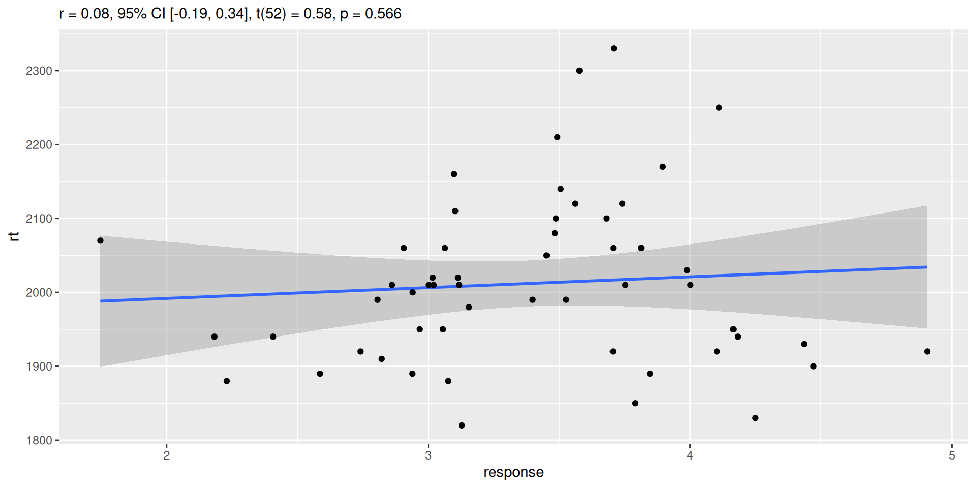
Parametric t-tests
One-sample t-test
t.test(my_data$response, mu = 3)
    One Sample t-test

data:  my_data$response
t = 4.5713, df = 53, p-value = 2.942e-05
alternative hypothesis: true mean is not equal to 3
95 percent confidence interval:
 3.216334 3.554596
sample estimates:
mean of x
 3.385465
Two-sample, independent t-test
Variance not assumed to be equal (default)
t.test(my_data_between$Young, my_data_between$Old) # works with columns
    Welch Two Sample t-test

data:  my_data_between$Young and my_data_between$Old
t = 1.8791, df = 14.815, p-value = 0.08005
alternative hypothesis: true difference in means is not equal to 0
95 percent confidence interval:
 -0.0705276  1.1113499
sample estimates:
mean of x mean of y
3.514574 2.994162 t.test(response ~ age, data = my_data1) # and with formulas
    Welch Two Sample t-test

data:  response by age
t = -1.8791, df = 14.815, p-value = 0.08005
alternative hypothesis: true difference in means between group Old and group Young is not equal to 0
95 percent confidence interval:
 -1.1113499  0.0705276
sample estimates:
  mean in group Old mean in group Young
           2.994162            3.514574
Two-sample, independent t-test
Student’s t-test with variance assumed equal
t.test(response ~ age, data = my_data1, var.equal = TRUE)
    Two Sample t-test

data:  response by age
t = -1.8791, df = 16, p-value = 0.07857
alternative hypothesis: true difference in means between group Old and group Young is not equal to 0
95 percent confidence interval:
 -1.10751153  0.06668926
sample estimates:
  mean in group Old mean in group Young
           2.994162            3.514574
Paired t-test
t.test(my_data_paired$time_1, my_data_paired$time_2, paired = TRUE) # works with columns
    Paired t-test

data:  my_data_paired$time_1 and my_data_paired$time_2
t = -1.7343, df = 17, p-value = 0.101
alternative hypothesis: true mean difference is not equal to 0
95 percent confidence interval:
 -0.67372926  0.06580605
sample estimates:
mean difference
     -0.3039616
Non-parametric t-tests
One-sample Wilcoxon signed rank test
wilcox.test(my_data$response, mu = 3)
    Wilcoxon signed rank test with continuity correction

data:  my_data$response
V = 1202, p-value = 7.747e-05
alternative hypothesis: true location is not equal to 3
Two-sample, independent Wilcoxon rank sum test
wilcox.test(my_data_between$Old, my_data_between$Young) # works with columns
    Wilcoxon rank sum exact test

data:  my_data_between$Old and my_data_between$Young
W = 19, p-value = 0.06253
alternative hypothesis: true location shift is not equal to 0wilcox.test(response ~ age, data = my_data1) # and with formulas
    Wilcoxon rank sum exact test

data:  response by age
W = 19, p-value = 0.06253
alternative hypothesis: true location shift is not equal to 0
Paired Wilcoxon signed rank test
wilcox.test(my_data_paired$time_1, my_data_paired$time_2, paired = TRUE) # works with columns
    Wilcoxon signed rank exact test

data:  my_data_paired$time_1 and my_data_paired$time_2
V = 49, p-value = 0.1187
alternative hypothesis: true location shift is not equal to 0
ANOVAs
Non-parametric (Kruskal-Wallis test)
kruskal.test(response ~ time, data = my_data)
    Kruskal-Wallis rank sum test

data:  response by time
Kruskal-Wallis chi-squared = 2.088, df = 2, p-value = 0.352
Factorial ANOVA
aov(response ~ gender, data = my_data)Call:
aov(formula = response ~ gender, data = my_data)
Terms:
gender Residuals
Sum of Squares 0.698464 19.651568
Deg. of Freedom 2 51
Residual standard error: 0.6207454
Estimated effects may be unbalanced Df Sum Sq Mean Sq F value Pr(>F)
gender 2 0.698 0.3492 0.906 0.41
Residuals 51 19.652 0.3853 Interaction
Main effect and interaction
            Df Sum Sq Mean Sq F value Pr(>F)
gender       2  0.698  0.3492   0.891  0.417
age          1  0.196  0.1959   0.500  0.483
gender:age   2  0.649  0.3245   0.828  0.443
Residuals   48 18.807  0.3918
# use * for both main effects and interaction
aov_test <- aov(response ~ gender * age, data = my_data)
summary(aov_test) Df Sum Sq Mean Sq F value Pr(>F)
gender 2 0.698 0.3492 0.891 0.417
age 1 0.196 0.1959 0.500 0.483
gender:age 2 0.649 0.3245 0.828 0.443
Residuals 48 18.807 0.3918 Post-hoc comparisons
{multcomp} package for more options
TukeyHSD(aov_test) Tukey multiple comparisons of means
95% family-wise confidence level
Fit: aov(formula = response ~ gender * age, data = my_data)
$gender
diff lwr upr p adj
Male-Female -0.21361569 -0.7182284 0.2909970 0.5656428
Nonbinary-Female 0.04805204 -0.4565606 0.5526647 0.9712021
Nonbinary-Male 0.26166774 -0.2429449 0.7662804 0.4278041
$age
diff lwr upr p adj
Young-Old 0.1204545 -0.222078 0.4629871 0.4829496
$`gender:age`
diff lwr upr p adj
Male:Old-Female:Old -0.299759805 -1.1755050 0.5759854 0.9103597
Nonbinary:Old-Female:Old 0.225248379 -0.6504968 1.1009936 0.9723190
Female:Young-Female:Old 0.181156021 -0.6945892 1.0569012 0.9894963
Male:Young-Female:Old 0.053684436 -0.8220608 0.9294297 0.9999705
Nonbinary:Young-Female:Old 0.052011732 -0.8237335 0.9277570 0.9999748
Nonbinary:Old-Male:Old 0.525008184 -0.3507370 1.4007534 0.4883543
Female:Young-Male:Old 0.480915826 -0.3948294 1.3566611 0.5834600
Male:Young-Male:Old 0.353444241 -0.5223010 1.2291895 0.8357157
Nonbinary:Young-Male:Old 0.351771537 -0.5239737 1.2275168 0.8384092
Female:Young-Nonbinary:Old -0.044092358 -0.9198376 0.8316529 0.9999889
Male:Young-Nonbinary:Old -0.171563943 -1.0473092 0.7041813 0.9918118
Nonbinary:Young-Nonbinary:Old -0.173236647 -1.0489819 0.7025086 0.9914384
Male:Young-Female:Young -0.127471585 -1.0032168 0.7482736 0.9979705
Nonbinary:Young-Female:Young -0.129144289 -1.0048895 0.7466009 0.9978402
Nonbinary:Young-Male:Young -0.001672704 -0.8774179 0.8740725 1.0000000Repeated measures ANOVA
Repeated measures ANOVA with interaction
Error: subject
    Df  Sum Sq Mean Sq
age  1 0.04394 0.04394

Error: Within
          Df Sum Sq Mean Sq F value Pr(>F)
age        1  0.159  0.1592   0.429  0.516
time       1  0.072  0.0718   0.193  0.662
age:time   1  1.878  1.8782   5.057  0.029 *
Residuals 49 18.197  0.3714
---
Signif. codes:  0 '***' 0.001 '**' 0.01 '*' 0.05 '.' 0.1 ' ' 1
{afex} package
Try {afex} for powerful ANOVA and linear modeling functions
library(afex)
aov_ez(id = "subject", dv = "response", between = "age",
       within = "time", data = my_data)
Anova Table (Type 3 tests)
Response: response
Effect df MSE F ges p.value
1 age 1, 16 0.33 0.60 .011 .451
2 time 1.88, 30.02 0.40 1.17 .048 .323
3 age:time 1.88, 30.02 0.40 2.61 + .102 .093
---
Signif. codes: 0 '***' 0.001 '**' 0.01 '*' 0.05 '+' 0.1 ' ' 1
Sphericity correction method: GG # by default, this uses type III sums of squares, like SPSSType II sums of squares
aov_ez(id = "subject", dv = "response", between = "age",
       within = "time", data = my_data, type = 2)
Anova Table (Type 2 tests)
Response: response
Effect df MSE F ges p.value
1 age 1, 16 0.33 0.60 .011 .451
2 time 1.88, 30.02 0.40 1.17 .048 .323
3 age:time 1.88, 30.02 0.40 2.61 + .102 .093
---
Signif. codes: 0 '***' 0.001 '**' 0.01 '*' 0.05 '+' 0.1 ' ' 1
Sphericity correction method: GG # but can set sums of squares, like II, which is what R uses by default