Grammar of graphics II
2025-03-31
Map data to visual properties
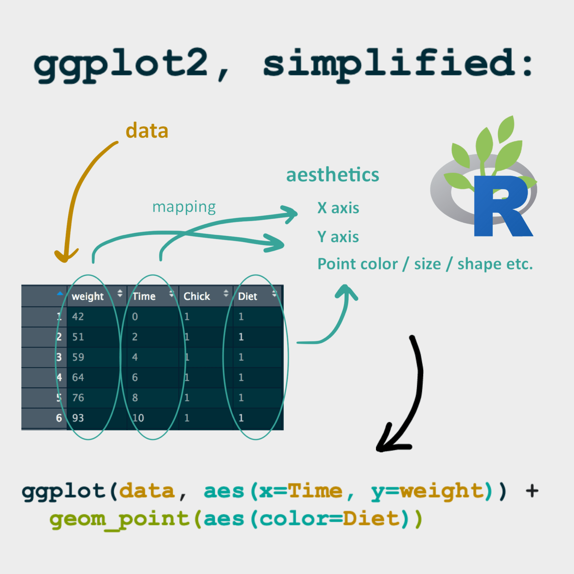
Map data columns to plot
mpg |>
  ggplot(aes(x = displ, y = hwy)) +
  geom_point()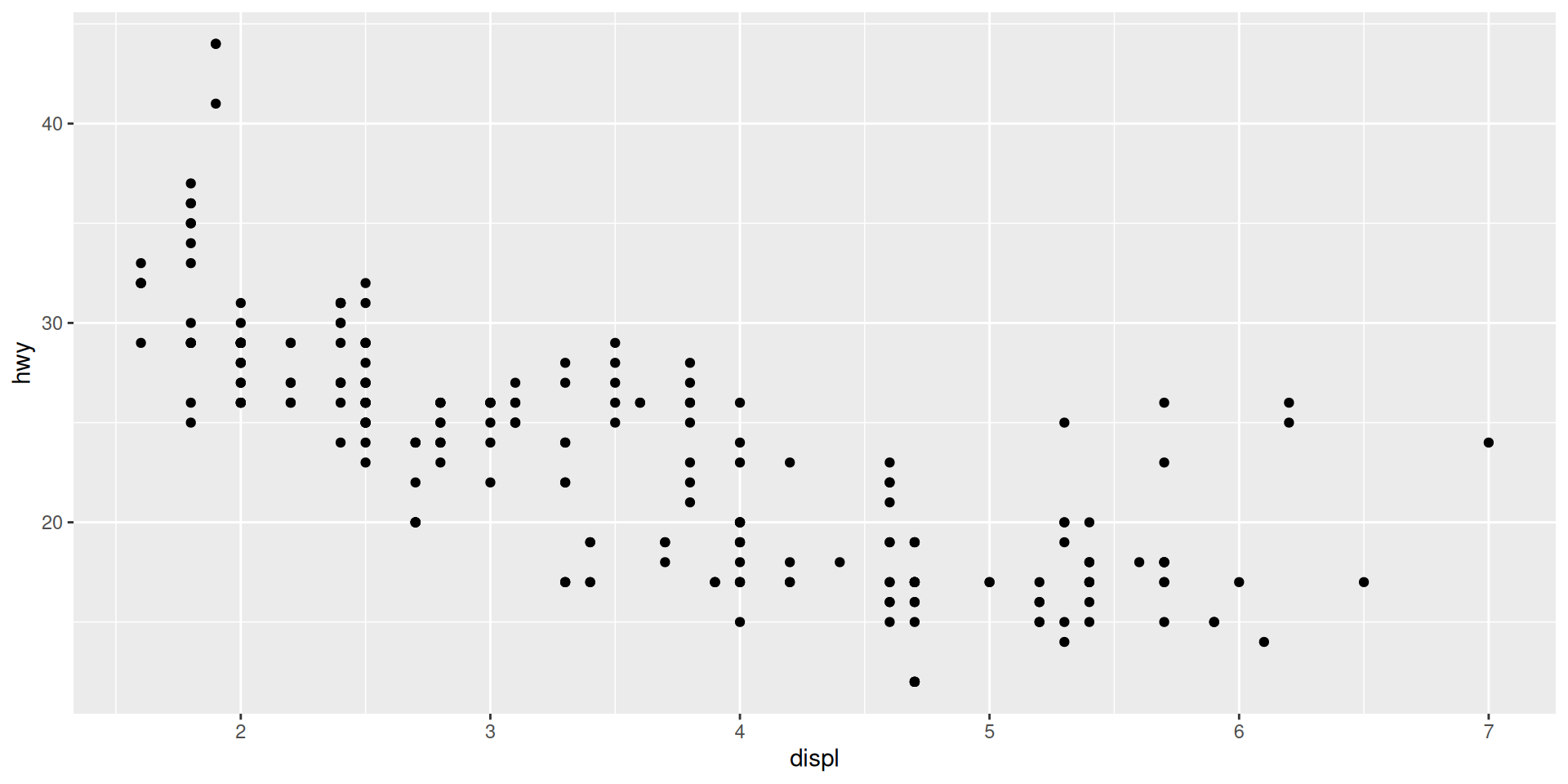
Size
Map data to aesthetic
mpg |>
  ggplot(aes(x = displ, y = hwy,
             size = cty)) +
  geom_point()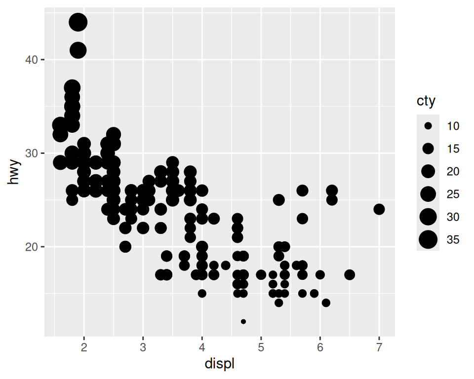
Apply to all points
mpg |>
  ggplot(aes(x = displ,
             y = hwy)) +
  geom_point(size = 0.5)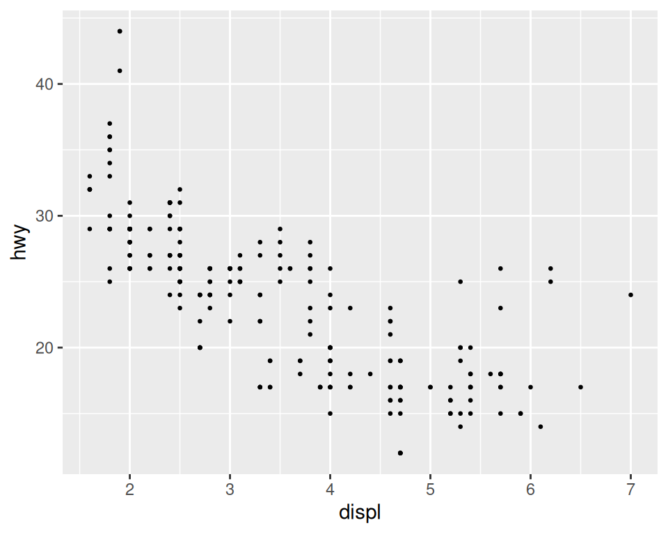
Transparency
mpg |>
  ggplot(aes(x = displ, y = hwy,
             alpha = cty)) +
  geom_point()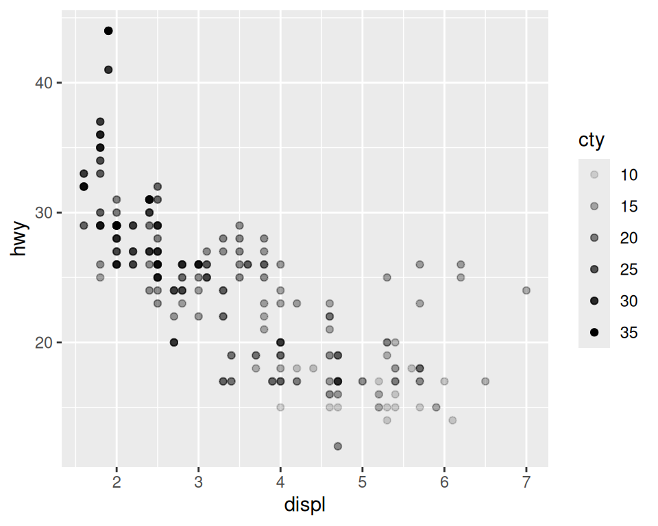
mpg |>
  ggplot(aes(x = displ,
             y = hwy)) +
  geom_point(alpha = 0.25)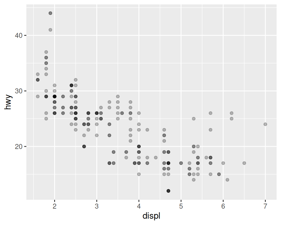
Shape
mpg |>
  ggplot(aes(x = displ, y = hwy,
             shape = class)) +
  geom_point()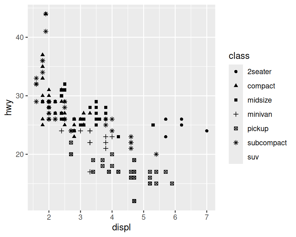
mpg |>
  ggplot(aes(x = displ,
             y = hwy)) +
  geom_point(shape = 5)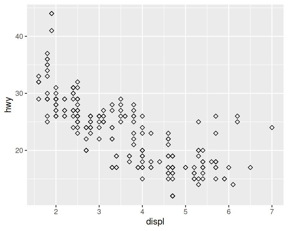
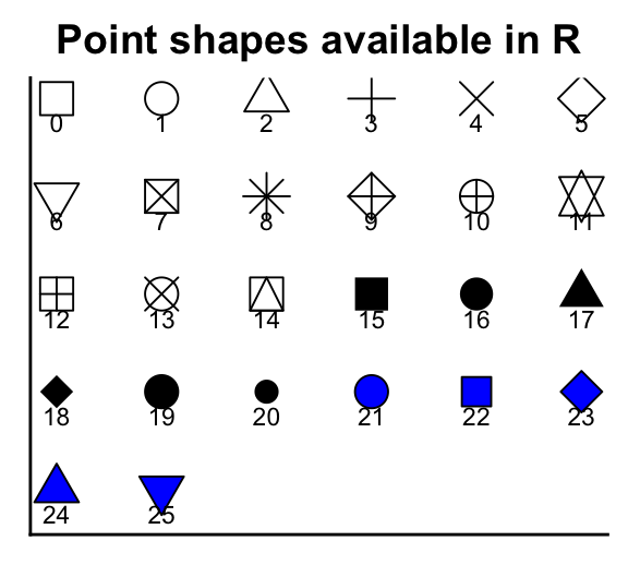
Shapes
Color
mpg |>
  ggplot(aes(x = displ, y = hwy,
             color = class)) +
  geom_point()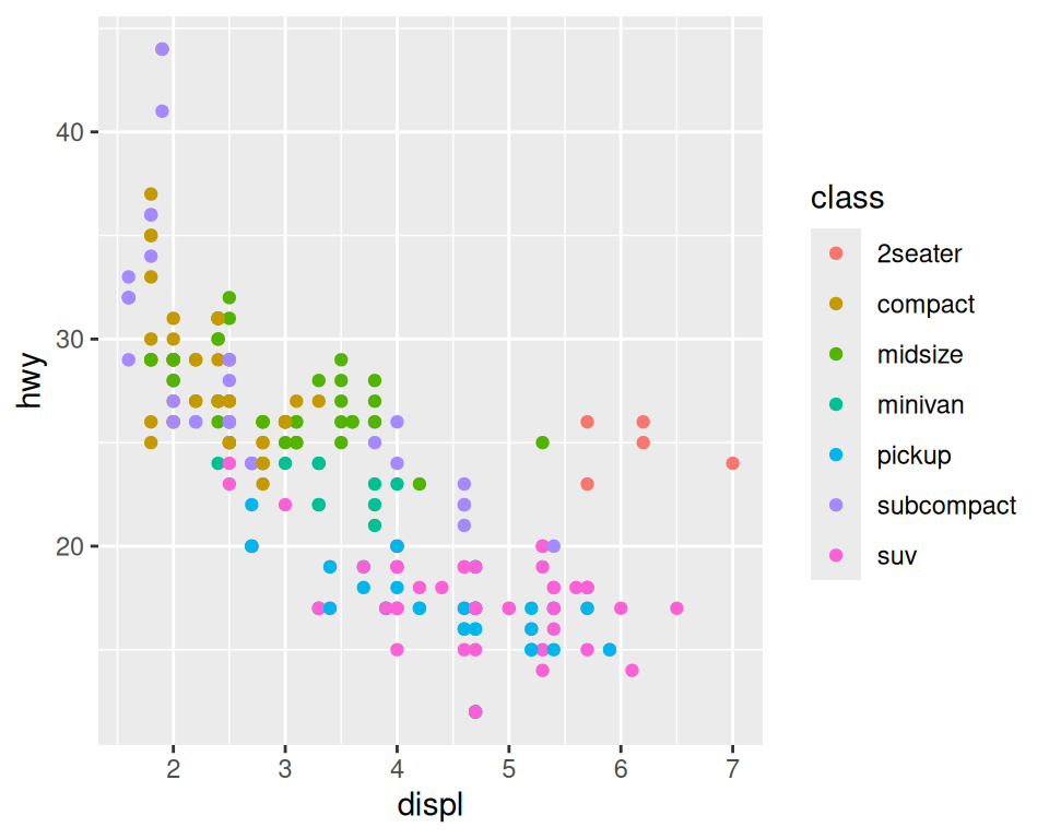
mpg |>
  ggplot(aes(x = displ,
             y = hwy)) +
  geom_point(color = "dodgerblue")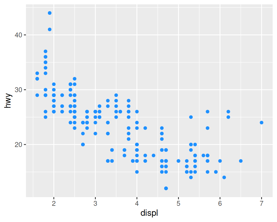
Color
What happens if we put a single color in the aesthetic?
mpg |>
  ggplot(aes(x = displ, y = hwy, color = "dodgerblue")) +
  geom_point()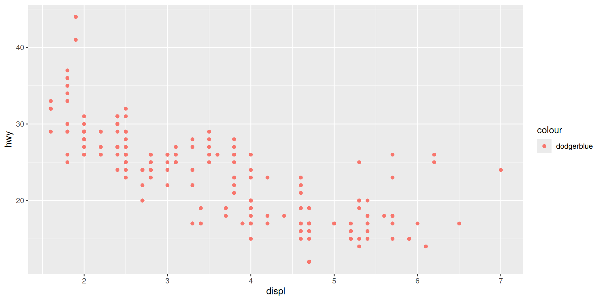
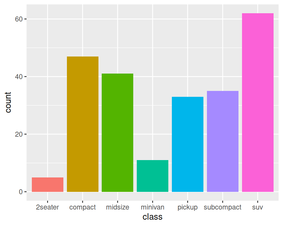
Color: points, lines, text, and borders
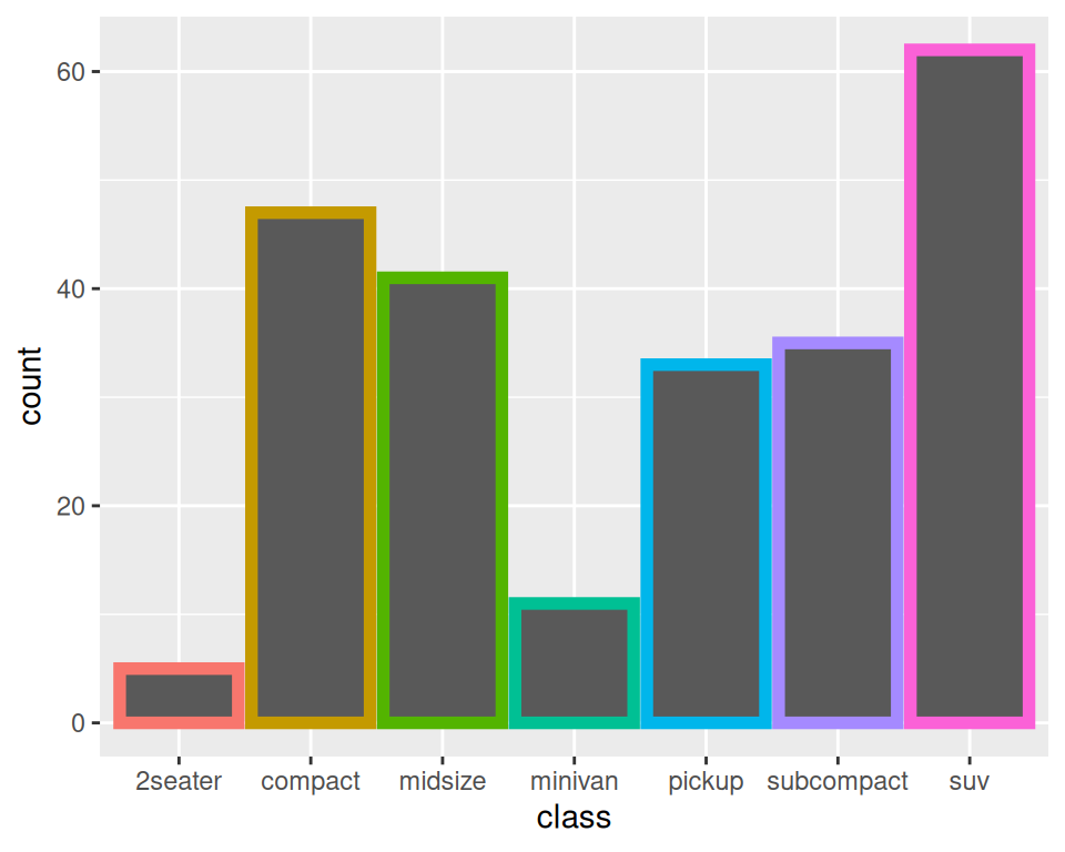
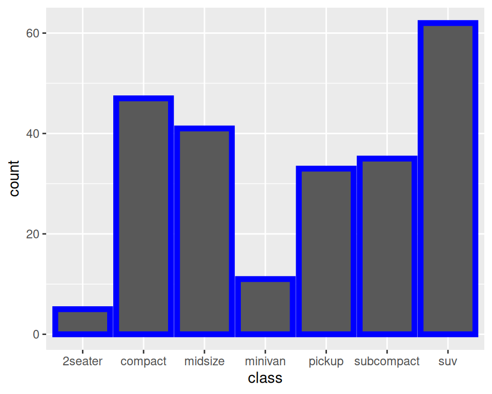
Fill: filled areas
Lines separated by groups
mpg |>
  ggplot(aes(x = displ, y = hwy, group = drv)) +
  geom_smooth()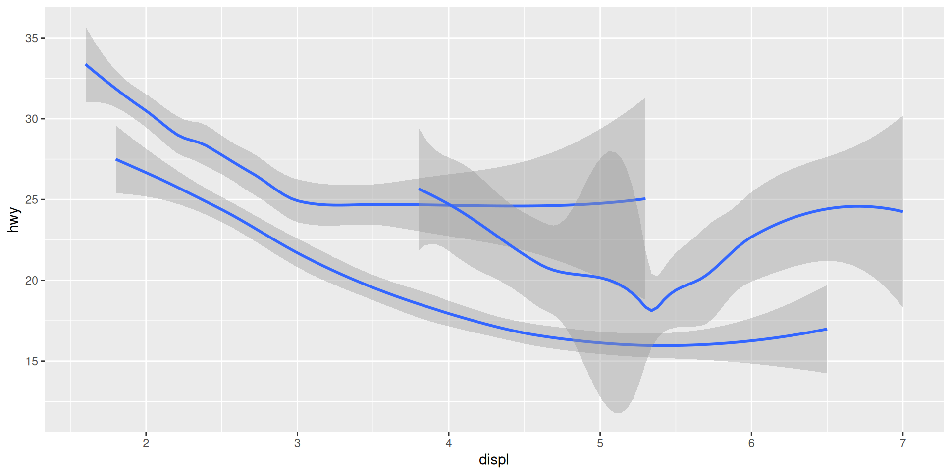
Linetype
mpg |>
  ggplot(aes(x = displ, y = hwy, linetype = drv)) +
  geom_smooth()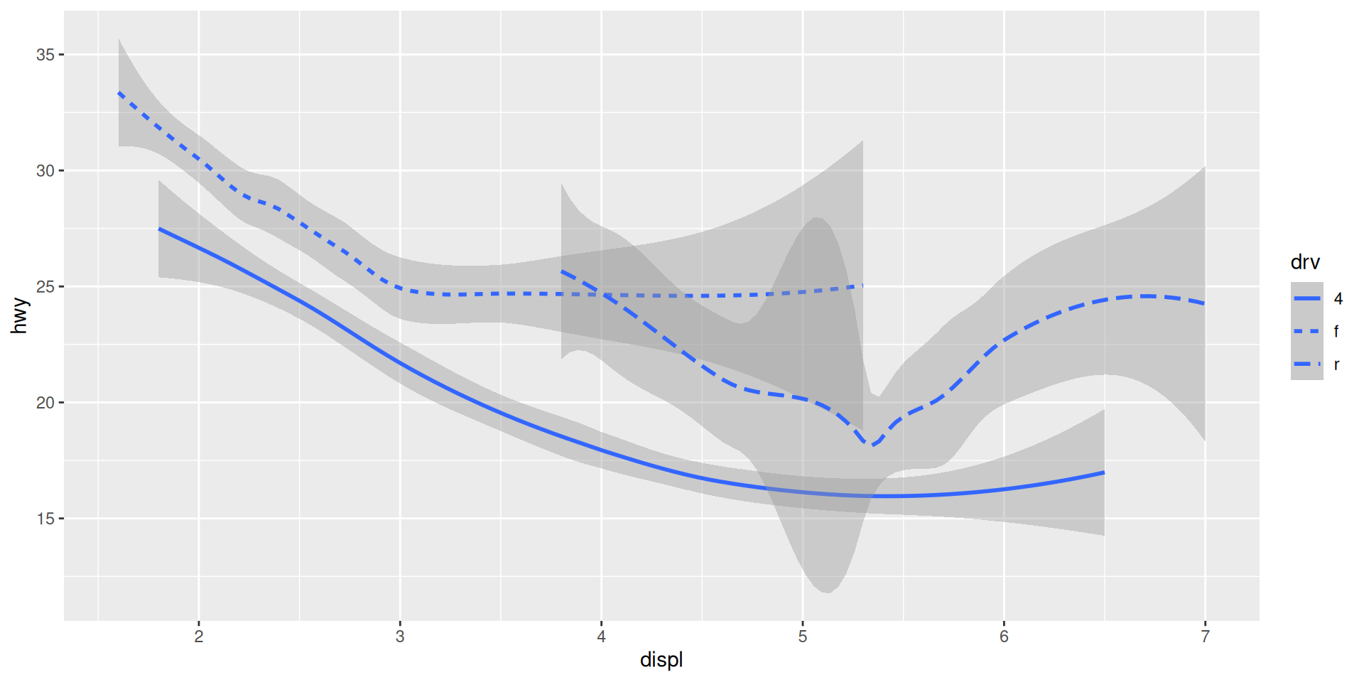
Apply line aesthetics to groups
mpg |>
  ggplot(aes(x = displ, y = hwy, color = drv)) +
  geom_smooth(show.legend = FALSE)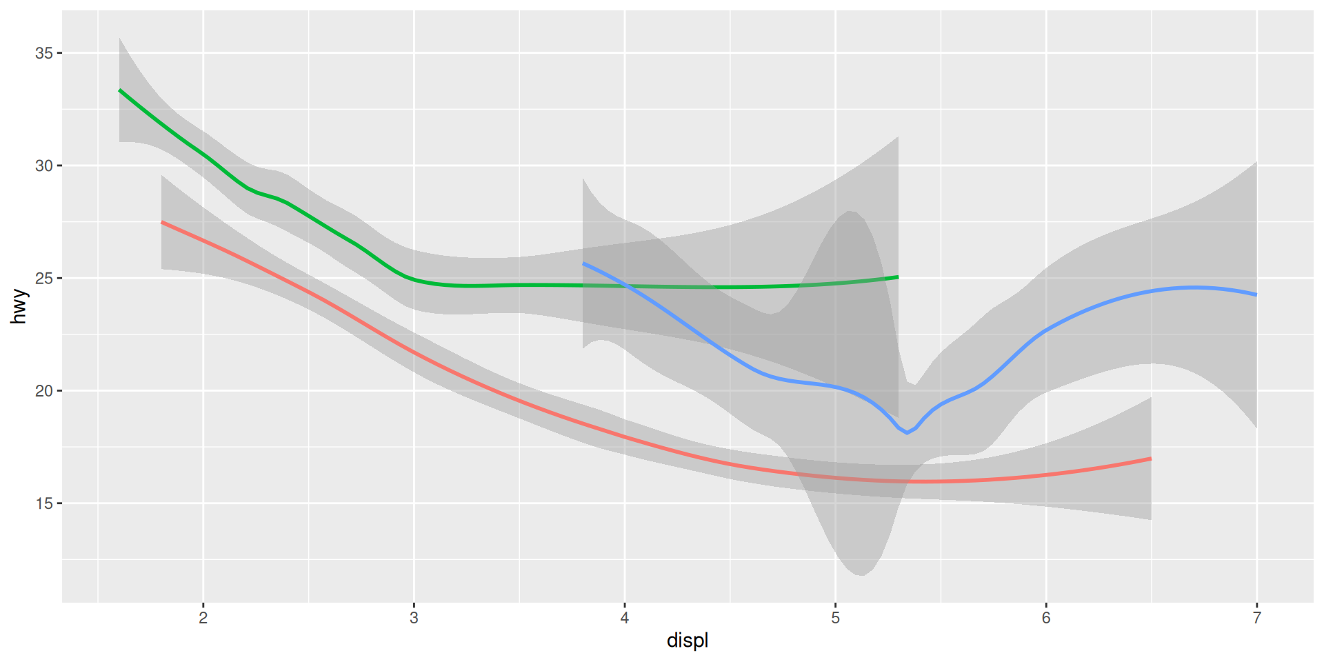
Apply aesthetics to one geom
mpg |>
  ggplot(aes(x = displ, y = hwy)) +
  geom_point(aes(color = class)) +
  geom_smooth()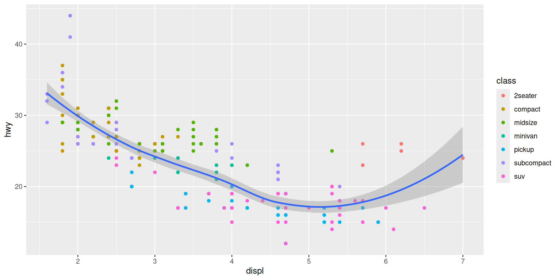
Apply aesthetics differently to geoms
mpg |>
  ggplot(aes(x = displ, y = hwy, color = drv)) +
  geom_point() +
  geom_smooth(aes(linetype = drv))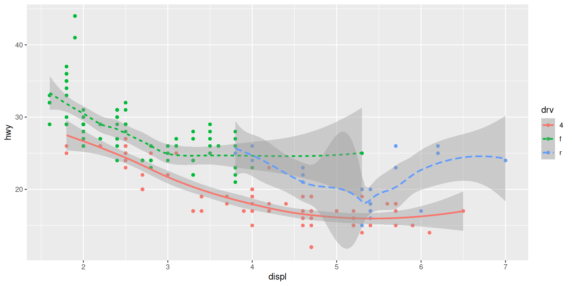
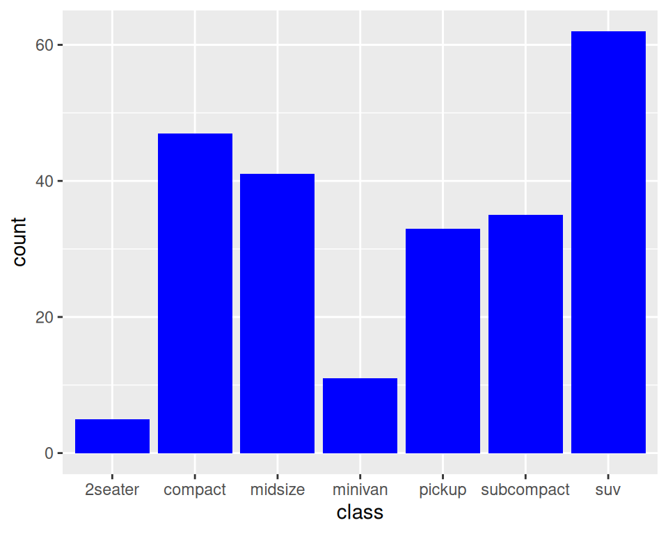
Bar plots
Count observations of variable types with stat_count()
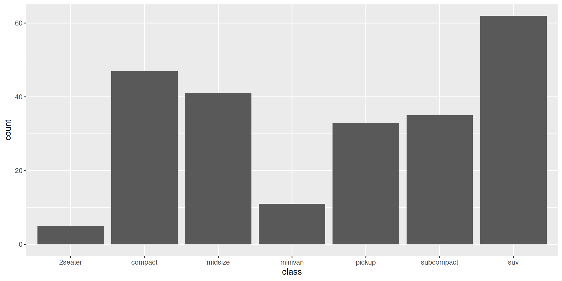
Summarize data with stat_summary()
mpg |>
  ggplot(aes(x = class, y = hwy)) +
  geom_point()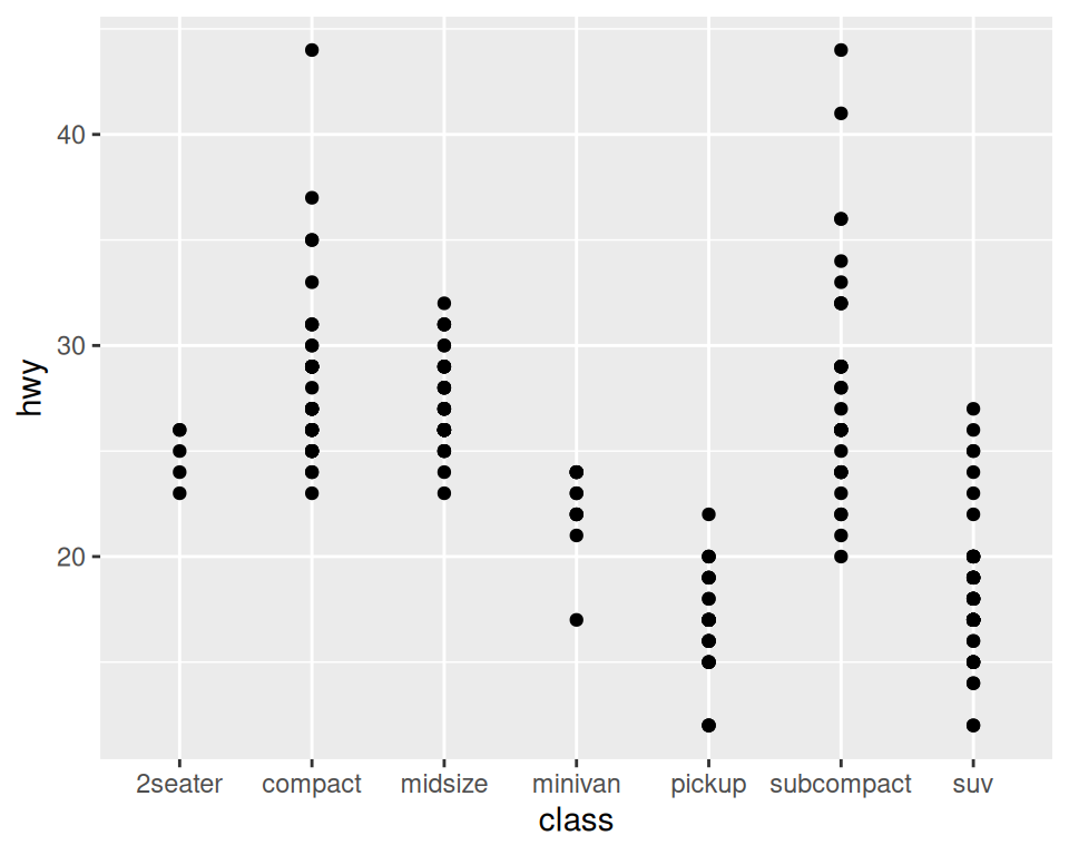
mpg |>
  ggplot(aes(x = class, y = hwy)) +
  stat_summary()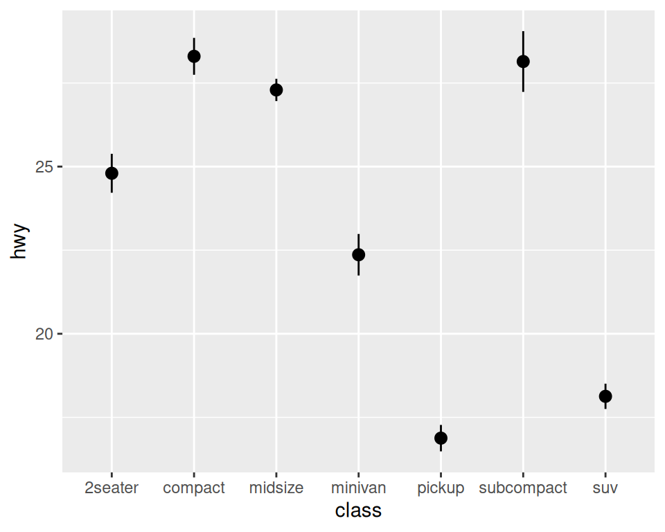
Summarize data
Plot mean and 95% CI
mpg |>
  ggplot(aes(x = class, y = hwy)) +
  stat_summary(fun.data = mean_cl_normal)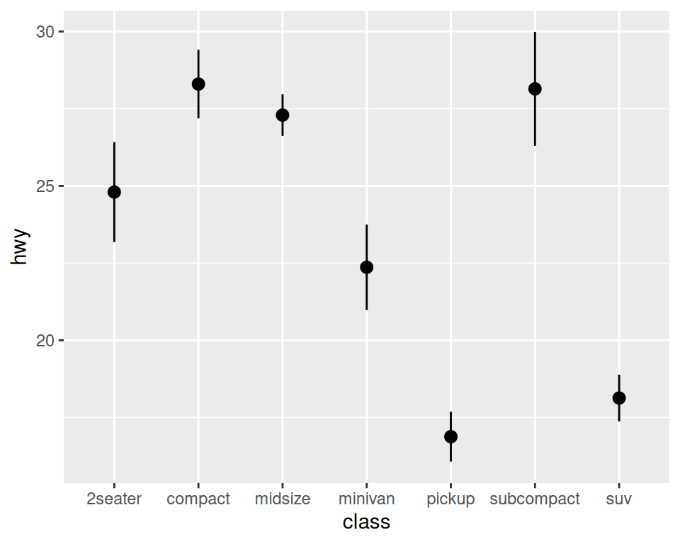
Plot median and range
mpg |>
  ggplot(aes(x = class, y = hwy)) +
  stat_summary(fun.min = min, fun.max = max, fun = median)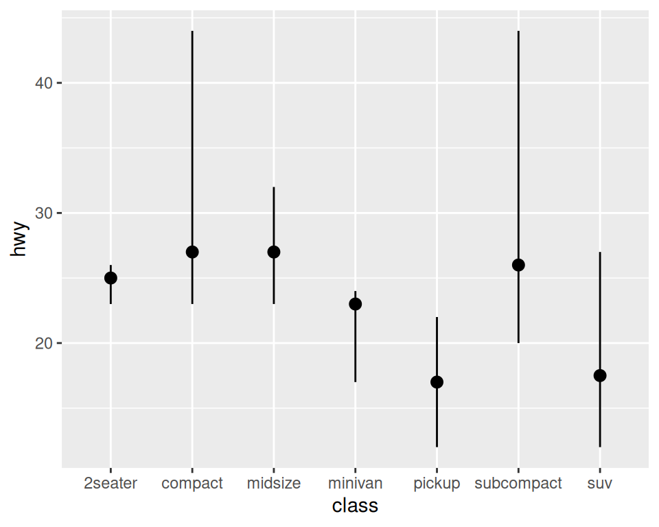
Visualizing groups
Coloring by group difficult to visualize with many groups
mpg |>
  ggplot(aes(x = displ, y = hwy, color = class)) +
  geom_point()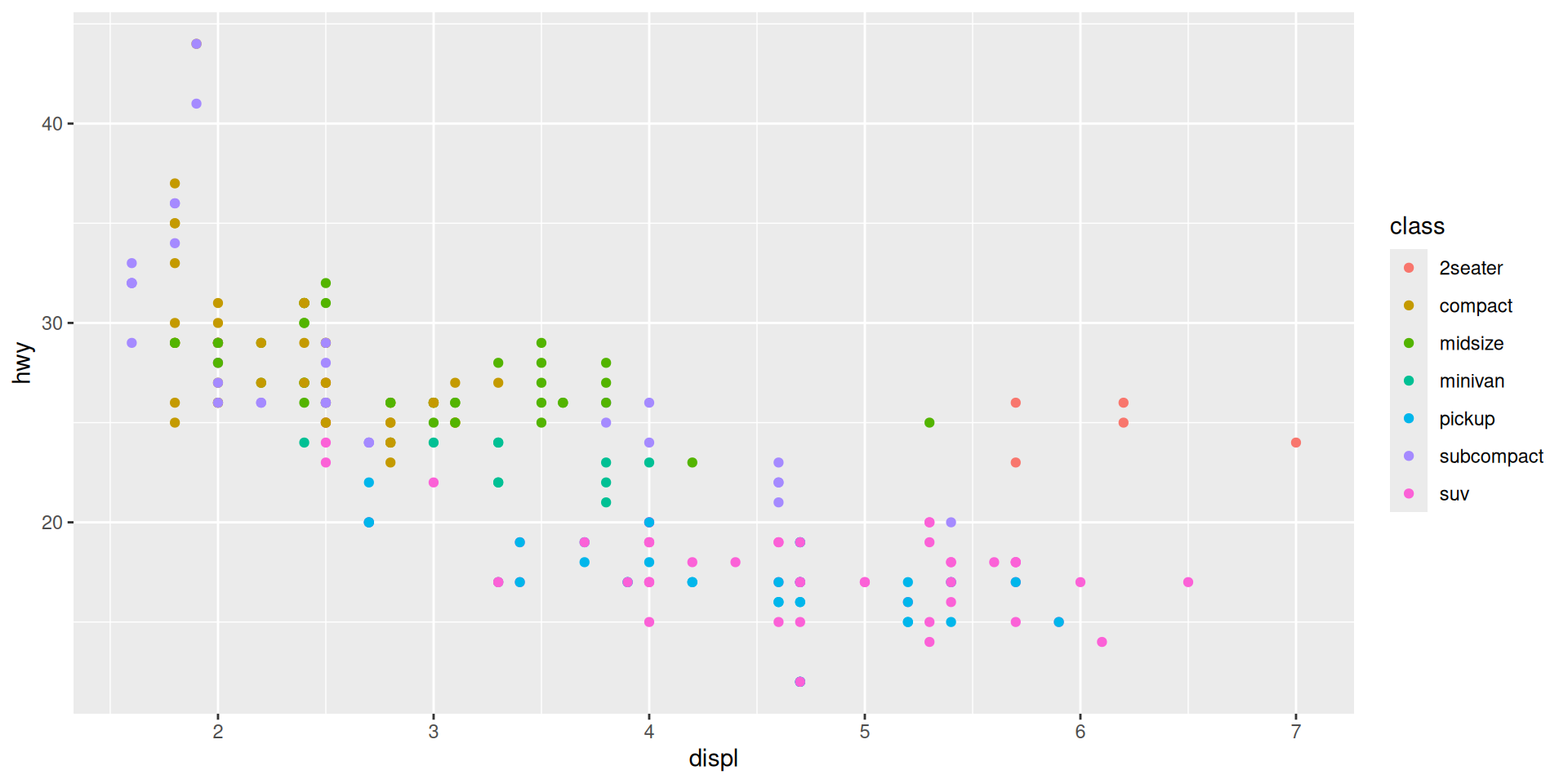
Faceting
Pulls out groups into separate panels
mpg |>
  ggplot(aes(x = displ, y = hwy)) +
  geom_point() +
  facet_wrap(vars(class))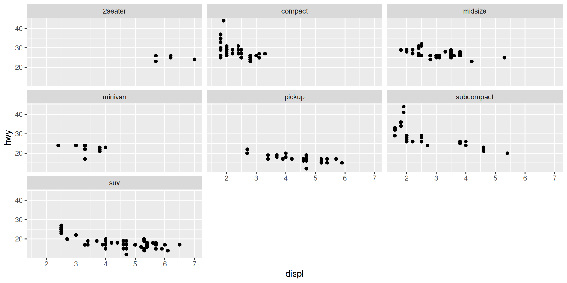
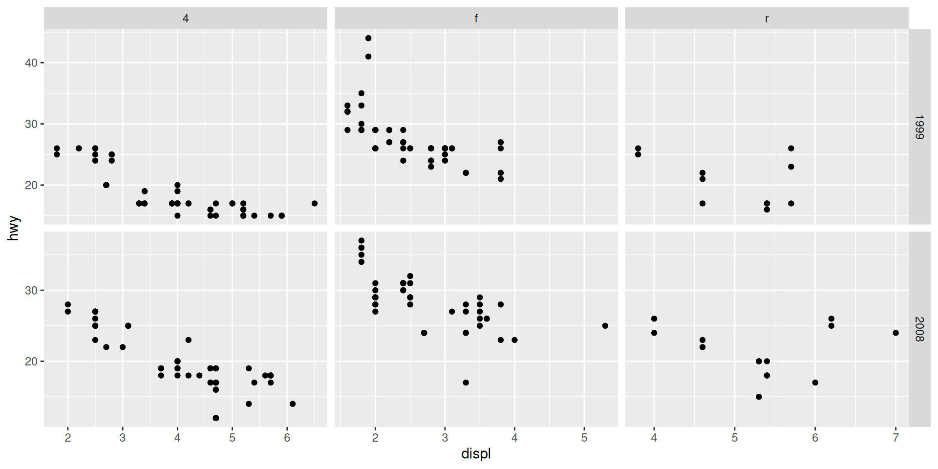
Faceting
Group by two or more variables with facet_grid()
mpg |>
  ggplot(aes(x = displ, y = hwy)) +
  geom_point() +
  facet_grid(rows = vars(year), cols = vars(drv))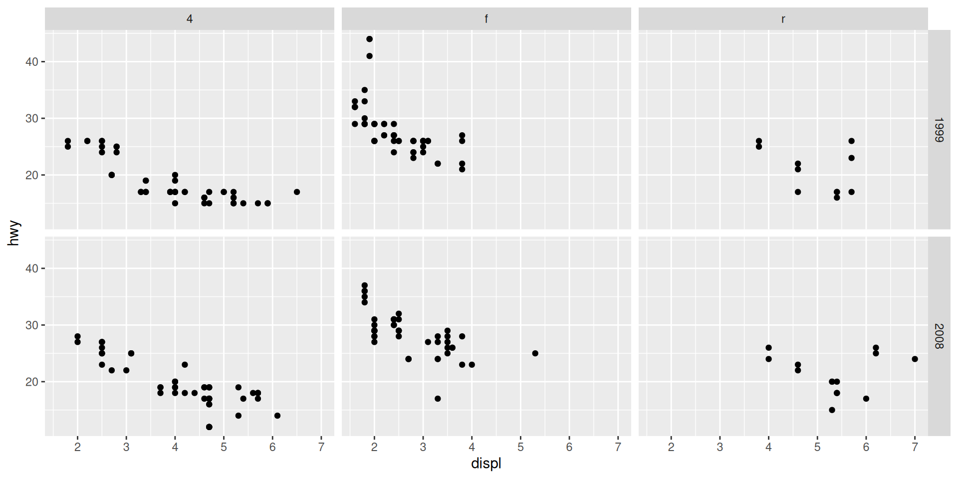
Faceting
Allow axes to vary with scales
mpg |>
  ggplot(aes(x = displ, y = hwy)) +
  geom_point() +
  facet_grid(rows = vars(year), cols = vars(drv),
             scales = "free_x")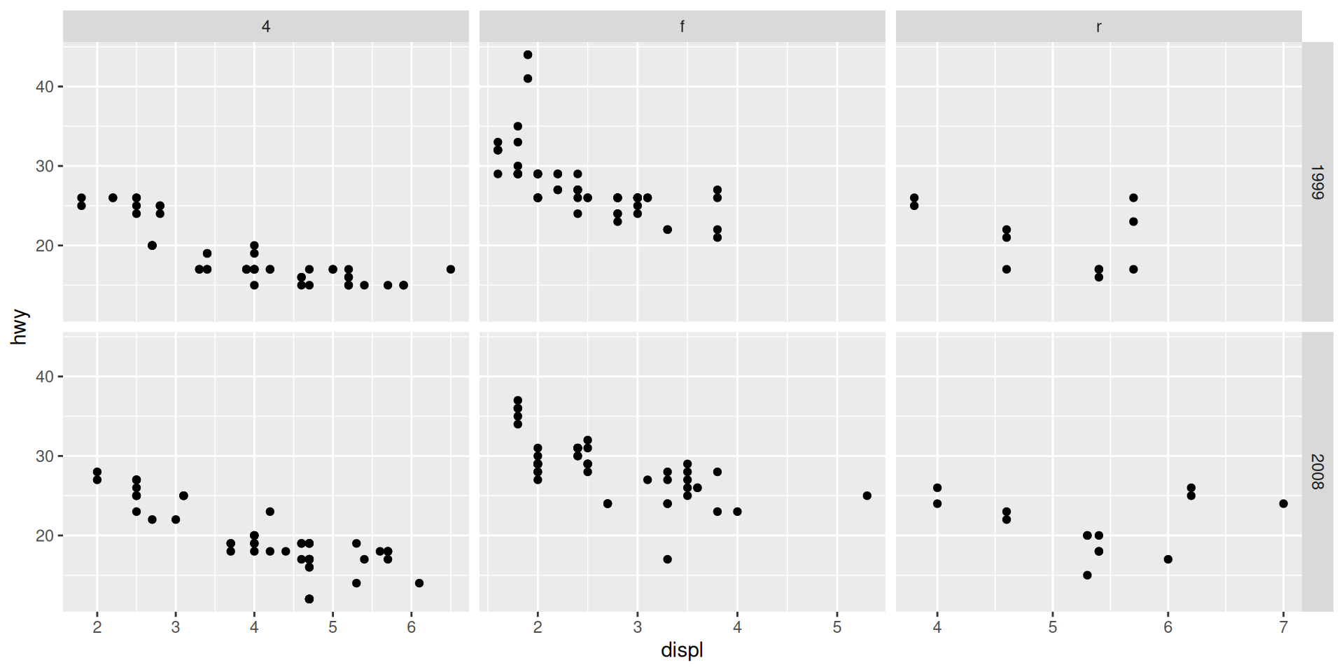
Facet
Allow axes to vary with scales
mpg |>
  ggplot(aes(x = displ, y = hwy)) +
  geom_point() +
  facet_grid(rows = vars(year), cols = vars(drv),
             scales = "free")