Numbers
Jeff Stevens
2025-03-05
Review
Group data wrangling challenge
Using the penguins data set from the {palmerpenguins} package, recreate this data frame.
# A tibble: 4 × 4
  species   island     male female
  <fct>     <fct>     <dbl>  <dbl>
1 Adelie    Torgersen 4035.  3396.
2 Adelie    Biscoe    4050   3369.
3 Adelie    Dream     4046.  3344.
4 Chinstrap Dream     3939.  3527.
Introduction
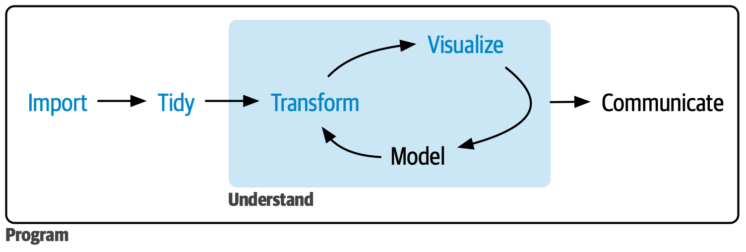
Mental model of data analysis
The problem
What’s different between these data sets?
What is needed to create data2 from data1?
data1# A tibble: 12 × 3
val1 val2 val3
<dbl> <dbl> <dbl>
1 0.372 0.129 0.00394
2 0.338 0.898 0.00925
3 0.889 0.324 0.00762
4 0.736 0.477 0.00902
5 0.493 0.928 0.00934
6 0.909 0.200 0.00142
7 0.650 0.846 0.00258
8 0.535 0.0300 0.00172
9 0.202 0.490 0.00329
10 0.613 0.649 0.00457
11 0.666 0.684 0.00325
12 0.510 0.356 0.00217data2# A tibble: 12 × 3
percent_val1 log_val2 val3
<dbl> <dbl> <chr>
1 37.2 -2.05 3.9e-03
2 33.8 -0.107 9.3e-03
3 88.9 -1.13 7.6e-03
4 73.6 -0.740 9.0e-03
5 49.3 -0.0747 9.3e-03
6 90.9 -1.61 1.4e-03
7 65.0 -0.167 2.6e-03
8 53.5 -3.51 1.7e-03
9 20.2 -0.713 3.3e-03
10 61.3 -0.432 4.6e-03
11 66.6 -0.379 3.3e-03
12 51 -1.03 2.2e-03Set-up
Comparing and counting
Comparing numbers
Counts
As a reminder, we’ve already seen how to use dplyr::count()
count(flights, carrier)# A tibble: 16 × 2
carrier n
<chr> <int>
1 9E 18460
2 AA 32729
3 AS 714
4 B6 54635
5 DL 48110
6 EV 54173
7 F9 685
8 FL 3260
9 HA 342
10 MQ 26397
11 OO 32
12 UA 58665
13 US 20536
14 VX 5162
15 WN 12275
16 YV 601Counts
We can also automatically sort by count.
count(flights, carrier, sort = TRUE)# A tibble: 16 × 2
carrier n
<chr> <int>
1 UA 58665
2 B6 54635
3 EV 54173
4 DL 48110
5 AA 32729
6 MQ 26397
7 US 20536
8 9E 18460
9 WN 12275
10 VX 5162
11 FL 3260
12 AS 714
13 F9 685
14 YV 601
15 HA 342
16 OO 32And sum up totals instead of just count
count(flights, carrier, wt = distance)# A tibble: 16 × 2
carrier n
<chr> <dbl>
1 9E 9788152
2 AA 43864584
3 AS 1715028
4 B6 58384137
5 DL 59507317
6 EV 30498951
7 F9 1109700
8 FL 2167344
9 HA 1704186
10 MQ 15033955
11 OO 16026
12 UA 89705524
13 US 11365778
14 VX 12902327
15 WN 12229203
16 YV 225395Counts
Remember n() counts inside a summarise()
n_distinct() counts instances within a group
flights |>
  group_by(dest) |>
  summarise(carriers =
              n_distinct(carrier))
# A tibble: 105 × 2
dest carriers
<chr> <int>
1 ABQ 1
2 ACK 1
3 ALB 1
4 ANC 1
5 ATL 7
6 AUS 6
7 AVL 2
8 BDL 2
9 BGR 2
10 BHM 1
# ℹ 95 more rowsCounting NAs
Counting NAs
This trick can be used for any logical vector
Transforming numbers
Mathematical transformations
 [1]  0.000000  3.162278  4.472136  5.477226  6.324555  7.071068  7.745967
[8] 8.366600 8.944272 9.486833 10.000000 [1] -1.65340685 -1.29070057 -1.07721774 -0.67318319 -0.16257538 -1.08017070
[7] -0.54354157 -0.04112082 -0.58662299 -1.58314303 [1] 0.6346852 1.0213321 0.8641012 0.3110083 1.1331782 1.0825151 1.2655997
[8] 0.3102413 1.0683179 1.1974808Rounding
Control significant digits with round()
Formatting numbers
Formatting
When numbers get too big, too small, or need other formatting, use format()
Cutting numbers into ranges
If you need to bin numbers into ranges, use cut()
 [1] 26.550866 37.212390 57.285336 90.820779 20.168193 89.838968 94.467527
[8] 66.079779 62.911404 6.178627 20.597457 17.655675 [1] (0,33] (33,66] (33,66] (66,100] (0,33] (66,100] (66,100] (66,100]
[9] (33,66] (0,33] (0,33] (0,33]
Levels: (0,33] (33,66] (66,100]Solving the problem
Solving the problem
data1# A tibble: 12 × 3
val1 val2 val3
<dbl> <dbl> <dbl>
1 0.372 0.129 0.00394
2 0.338 0.898 0.00925
3 0.889 0.324 0.00762
4 0.736 0.477 0.00902
5 0.493 0.928 0.00934
6 0.909 0.200 0.00142
7 0.650 0.846 0.00258
8 0.535 0.0300 0.00172
9 0.202 0.490 0.00329
10 0.613 0.649 0.00457
11 0.666 0.684 0.00325
12 0.510 0.356 0.00217data2# A tibble: 12 × 3
percent_val1 log_val2 val3
<dbl> <dbl> <chr>
1 37.2 -2.05 3.9e-03
2 33.8 -0.107 9.3e-03
3 88.9 -1.13 7.6e-03
4 73.6 -0.740 9.0e-03
5 49.3 -0.0747 9.3e-03
6 90.9 -1.61 1.4e-03
7 65.0 -0.167 2.6e-03
8 53.5 -3.51 1.7e-03
9 20.2 -0.713 3.3e-03
10 61.3 -0.432 4.6e-03
11 66.6 -0.379 3.3e-03
12 51 -1.03 2.2e-03