Merging rows

Jeff Stevens

2025-03-03

Introduction

The problem

What’s different between these data sets?

What is needed to create data3 from data1 and data2?

data1

# A tibble: 12 × 2
      id   resp
   <int>  <dbl>
 1     1 0.130 
 2     2 0.992 
 3     3 0.947 
 4     4 0.0274
 5     5 0.705 
 6     6 0.0499
 7     7 0.874 
 8     8 0.742 
 9     9 0.240 
10    10 0.330 
11    11 0.379 
12    12 0.174

data2

# A tibble: 12 × 2
      id  cond
   <int> <int>
 1     1     1
 2     2     2
 3     3     3
 4     4     1
 5     5     2
 6     6     3
 7     7     1
 8     8     2
 9     9     3
10    10     1
11    11     2
12    12     3

data3

# A tibble: 4 × 2
     id   resp
  <int>  <dbl>
1     1 0.130 
2     4 0.0274
3     7 0.874 
4    10 0.330

Set-up

library(dplyr)
library(nycflights13)
(flights2 <- select(flights, year:dep_time, carrier, tailnum))

# A tibble: 336,776 × 6
    year month   day dep_time carrier tailnum
   <int> <int> <int>    <int> <chr>   <chr>  
 1  2013     1     1      517 UA      N14228 
 2  2013     1     1      533 UA      N24211 
 3  2013     1     1      542 AA      N619AA 
 4  2013     1     1      544 B6      N804JB 
 5  2013     1     1      554 DL      N668DN 
 6  2013     1     1      554 UA      N39463 
 7  2013     1     1      555 B6      N516JB 
 8  2013     1     1      557 EV      N829AS 
 9  2013     1     1      557 B6      N593JB 
10  2013     1     1      558 AA      N3ALAA 
# ℹ 336,766 more rows

Set-up

set.seed(20250303)
(airlines2 <- slice_sample(airlines, prop = 0.5))

# A tibble: 8 × 2
  carrier name                       
  <chr>   <chr>                      
1 HA      Hawaiian Airlines Inc.     
2 MQ      Envoy Air                  
3 9E      Endeavor Air Inc.          
4 AA      American Airlines Inc.     
5 FL      AirTran Airways Corporation
6 B6      JetBlue Airways            
7 EV      ExpressJet Airlines Inc.   
8 UA      United Air Lines Inc.

(airlines3 <- rename(airlines2, airline = carrier))

# A tibble: 8 × 2
  airline name                       
  <chr>   <chr>                      
1 HA      Hawaiian Airlines Inc.     
2 MQ      Envoy Air                  
3 9E      Endeavor Air Inc.          
4 AA      American Airlines Inc.     
5 FL      AirTran Airways Corporation
6 B6      JetBlue Airways            
7 EV      ExpressJet Airlines Inc.   
8 UA      United Air Lines Inc.

Joining with {dplyr}

library(dplyr)

Filtering joins

Filters rows

Semi joins

Keep only matching observations

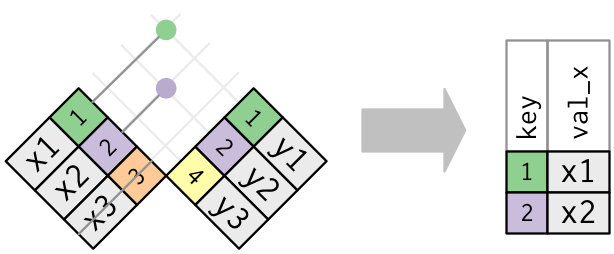
When is this useful?

Semi joins

# A tibble: 3 × 2
    key val_x
  <dbl> <chr>
1     1 x1   
2     2 x2   
3     3 x3

# A tibble: 3 × 2
    key val_y
  <dbl> <chr>
1     1 y1   
2     2 y2   
3     4 y3

semi_join(x, y, by = "key")

# A tibble: 2 × 2
    key val_x
  <dbl> <chr>
1     1 x1   
2     2 x2

Semi joins

airlines2

# A tibble: 8 × 2
  carrier name                       
  <chr>   <chr>                      
1 HA      Hawaiian Airlines Inc.     
2 MQ      Envoy Air                  
3 9E      Endeavor Air Inc.          
4 AA      American Airlines Inc.     
5 FL      AirTran Airways Corporation
6 B6      JetBlue Airways            
7 EV      ExpressJet Airlines Inc.   
8 UA      United Air Lines Inc.

Semi joins

flights2 |>
  semi_join(airlines2, by = "carrier")

# A tibble: 248,661 × 6
    year month   day dep_time carrier tailnum
   <int> <int> <int>    <int> <chr>   <chr>  
 1  2013     1     1      517 UA      N14228 
 2  2013     1     1      533 UA      N24211 
 3  2013     1     1      542 AA      N619AA 
 4  2013     1     1      544 B6      N804JB 
 5  2013     1     1      554 UA      N39463 
 6  2013     1     1      555 B6      N516JB 
 7  2013     1     1      557 EV      N829AS 
 8  2013     1     1      557 B6      N593JB 
 9  2013     1     1      558 AA      N3ALAA 
10  2013     1     1      558 B6      N793JB 
# ℹ 248,651 more rows

Semi joins

How could we do this with filter()?

flights2 |>
  filter(carrier %in% airlines2$carrier)

# A tibble: 248,661 × 6
    year month   day dep_time carrier tailnum
   <int> <int> <int>    <int> <chr>   <chr>  
 1  2013     1     1      517 UA      N14228 
 2  2013     1     1      533 UA      N24211 
 3  2013     1     1      542 AA      N619AA 
 4  2013     1     1      544 B6      N804JB 
 5  2013     1     1      554 UA      N39463 
 6  2013     1     1      555 B6      N516JB 
 7  2013     1     1      557 EV      N829AS 
 8  2013     1     1      557 B6      N593JB 
 9  2013     1     1      558 AA      N3ALAA 
10  2013     1     1      558 B6      N793JB 
# ℹ 248,651 more rows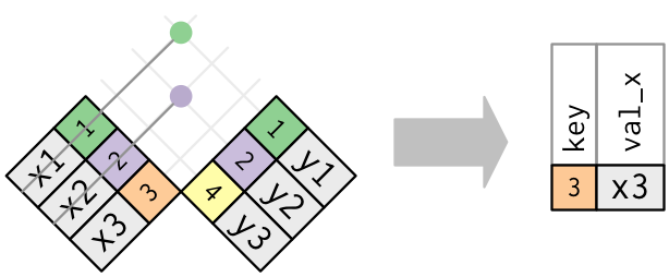

Anti joins

Keep only non-matching observations

When is this useful?

Anti joins

# A tibble: 3 × 2
    key val_x
  <dbl> <chr>
1     1 x1   
2     2 x2   
3     3 x3

# A tibble: 3 × 2
    key val_y
  <dbl> <chr>
1     1 y1   
2     2 y2   
3     4 y3

anti_join(x, y, by = "key")

# A tibble: 1 × 2
    key val_x
  <dbl> <chr>
1     3 x3

Anti joins

flights2 |>
  anti_join(airlines2, by = "carrier")

# A tibble: 88,115 × 6
    year month   day dep_time carrier tailnum
   <int> <int> <int>    <int> <chr>   <chr>  
 1  2013     1     1      554 DL      N668DN 
 2  2013     1     1      602 DL      N971DL 
 3  2013     1     1      606 DL      N3739P 
 4  2013     1     1      615 DL      N326NB 
 5  2013     1     1      622 US      N807AW 
 6  2013     1     1      627 US      N535UW 
 7  2013     1     1      629 WN      N273WN 
 8  2013     1     1      629 US      N426US 
 9  2013     1     1      643 US      N178US 
10  2013     1     1      653 DL      N327NW 
# ℹ 88,105 more rows

Anti joins

How could we do this with filter()?

flights2 |>
  filter(!carrier %in% airlines2$carrier)

# A tibble: 88,115 × 6
    year month   day dep_time carrier tailnum
   <int> <int> <int>    <int> <chr>   <chr>  
 1  2013     1     1      554 DL      N668DN 
 2  2013     1     1      602 DL      N971DL 
 3  2013     1     1      606 DL      N3739P 
 4  2013     1     1      615 DL      N326NB 
 5  2013     1     1      622 US      N807AW 
 6  2013     1     1      627 US      N535UW 
 7  2013     1     1      629 WN      N273WN 
 8  2013     1     1      629 US      N426US 
 9  2013     1     1      643 US      N178US 
10  2013     1     1      653 DL      N327NW 
# ℹ 88,105 more rows

Binding rows and columns

Adding rows

tibble::add_row()

(df <- tibble(x = 1:3, y = 3:1))

# A tibble: 3 × 2
      x     y
  <int> <int>
1     1     3
2     2     2
3     3     1

df |> add_row(x = 4, y = 0)

# A tibble: 4 × 2
      x     y
  <dbl> <dbl>
1     1     3
2     2     2
3     3     1
4     4     0

df |> add_row(x = 4, y = 0, 
               .before = 2)

# A tibble: 4 × 2
      x     y
  <dbl> <dbl>
1     1     3
2     4     0
3     2     2
4     3     1

df |> add_row(x = 4:5, y = 0:-1)

# A tibble: 5 × 2
      x     y
  <int> <int>
1     1     3
2     2     2
3     3     1
4     4     0
5     5    -1

Adding columns

tibble::add_column()

(df <- tibble(x = 1:3, y = 3:1))

# A tibble: 3 × 2
      x     y
  <int> <int>
1     1     3
2     2     2
3     3     1

df |> add_column(z = 4:6)

# A tibble: 3 × 3
      x     y     z
  <int> <int> <int>
1     1     3     4
2     2     2     5
3     3     1     6

df |> add_column(w = 4:6, 
                  .before = 1)

# A tibble: 3 × 3
      w     x     y
  <int> <int> <int>
1     4     1     3
2     5     2     2
3     6     3     1

df |> add_column(z = 4:6, alpha = 0)

# A tibble: 3 × 4
      x     y     z alpha
  <int> <int> <int> <dbl>
1     1     3     4     0
2     2     2     5     0
3     3     1     6     0

Combine data frames by rows

dplyr::bind_rows()

(df2 <- tibble(x = 4:5, y = 5:4))

# A tibble: 2 × 2
      x     y
  <int> <int>
1     4     5
2     5     4

bind_rows(df, df2)

# A tibble: 5 × 2
      x     y
  <int> <int>
1     1     3
2     2     2
3     3     1
4     4     5
5     5     4

(df3 <- tibble(y = 7:6, x = 6:7, 
               z = c("A", "B")))

# A tibble: 2 × 3
      y     x z    
  <int> <int> <chr>
1     7     6 A    
2     6     7 B

bind_rows(df, df3)

# A tibble: 5 × 3
      x     y z    
  <int> <int> <chr>
1     1     3 <NA> 
2     2     2 <NA> 
3     3     1 <NA> 
4     6     7 A    
5     7     6 B

Combine data frames by columns

dplyr::bind_cols()

(df4 <- tibble(z = c("A", "B" , "C"), 
               zz = c("Z", "Y", "X")))

# A tibble: 3 × 2
  z     zz   
  <chr> <chr>
1 A     Z    
2 B     Y    
3 C     X

bind_cols(df, df4)

# A tibble: 3 × 4
      x     y z     zz   
  <int> <int> <chr> <chr>
1     1     3 A     Z    
2     2     2 B     Y    
3     3     1 C     X

bind_cols(df, new_col = df4$z)

# A tibble: 3 × 3
      x     y new_col
  <int> <int> <chr>  
1     1     3 A      
2     2     2 B      
3     3     1 C

But why is this dangerous? What is a better solution?

Set operations

For finding overlap, differences, and combinations in values of datasets (apply to vectors and data frames)

Intersect

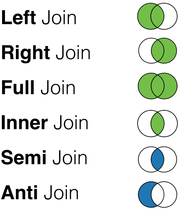
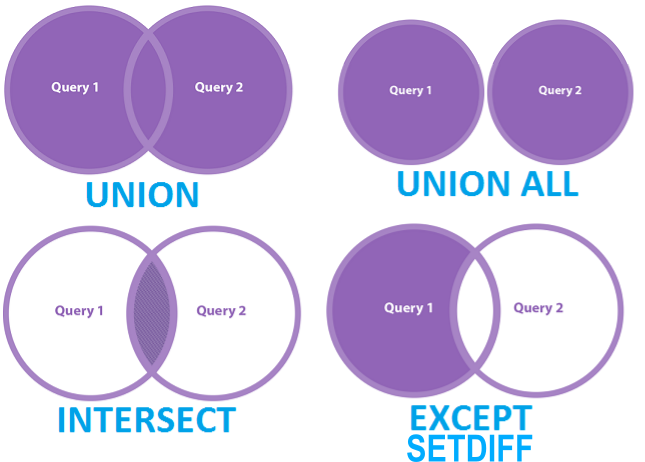
Common rows in both x and y, keeping just overlapping rows

Set difference

All rows from x which are not also rows in y, keeping just unique rows

Union

All unique rows from x and y

SQL

Congratulations—you just learned SQL databases!

Solving the problem

library(tidyverse)
nrows <- 12
set.seed(20250303)
data1 <- tibble(id = 1:nrows, resp = round(runif(nrows), nrows))
data2 <- tibble(id = 1:nrows, cond = rep(1:3, times = 4))

Solving the problem

What code combines data1 and data2 into data3?

data1

# A tibble: 12 × 2
      id   resp
   <int>  <dbl>
 1     1 0.130 
 2     2 0.992 
 3     3 0.947 
 4     4 0.0274
 5     5 0.705 
 6     6 0.0499
 7     7 0.874 
 8     8 0.742 
 9     9 0.240 
10    10 0.330 
11    11 0.379 
12    12 0.174

data2

# A tibble: 12 × 2
      id  cond
   <int> <int>
 1     1     1
 2     2     2
 3     3     3
 4     4     1
 5     5     2
 6     6     3
 7     7     1
 8     8     2
 9     9     3
10    10     1
11    11     2
12    12     3

data3

# A tibble: 4 × 2
     id   resp
  <int>  <dbl>
1     1 0.130 
2     4 0.0274
3     7 0.874 
4    10 0.330

Let’s code!

Merging rows