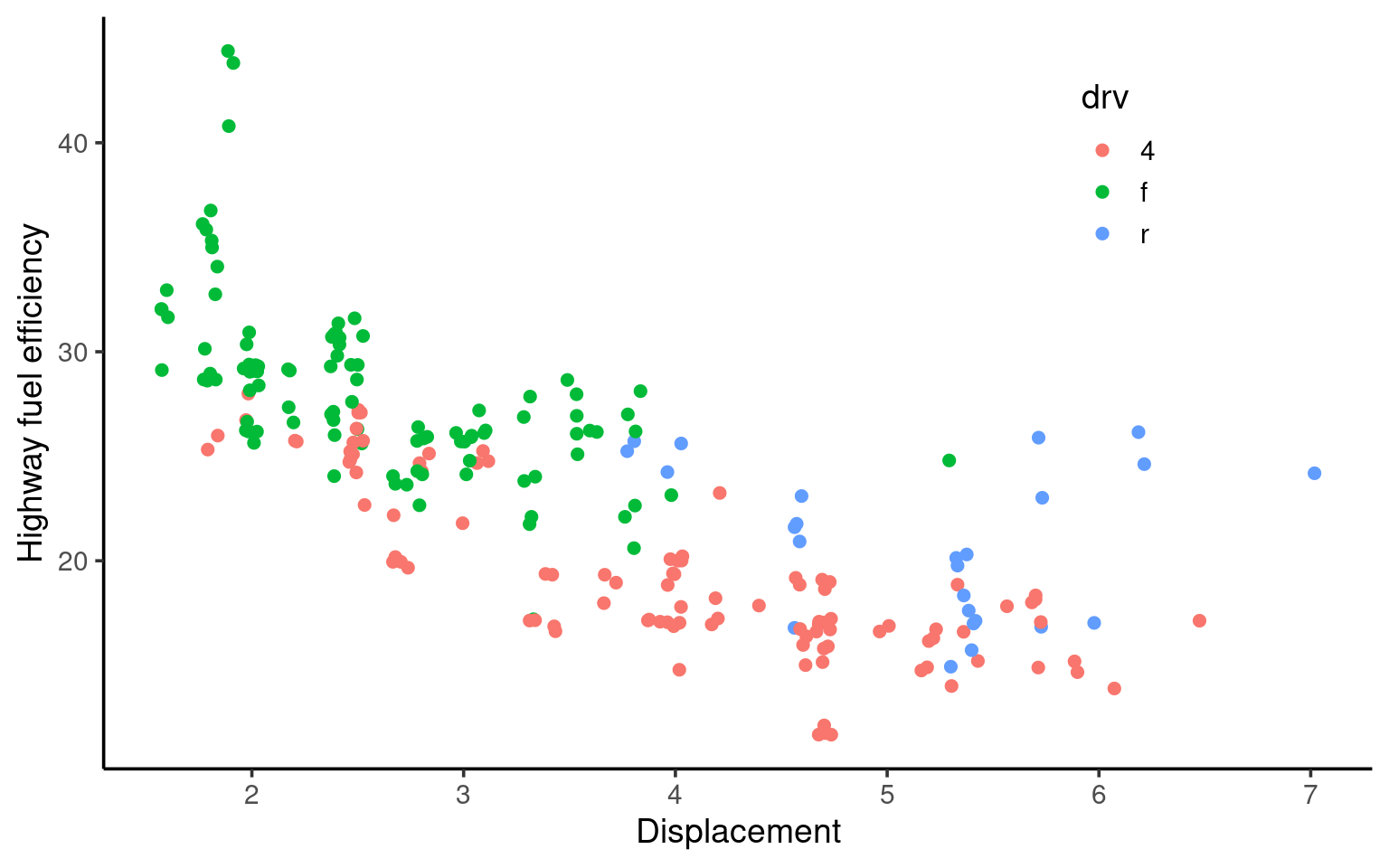


mpg |>
  ggplot(aes(x = displ, y = hwy, color = drv)) +
  geom_jitter() +
  labs(x = "Displacement", y = "Highway fuel efficiency") +
  scale_color_brewer(palette = "Accent") +
  theme(legend.position = c(0.8, 0.8))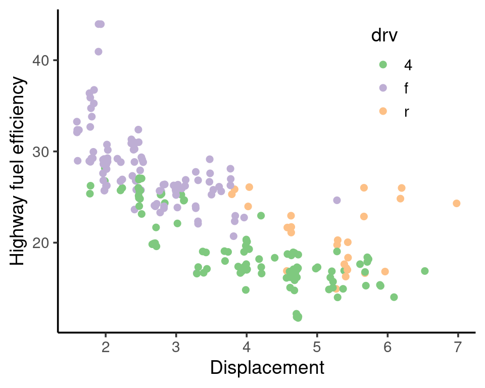
2023-04-07
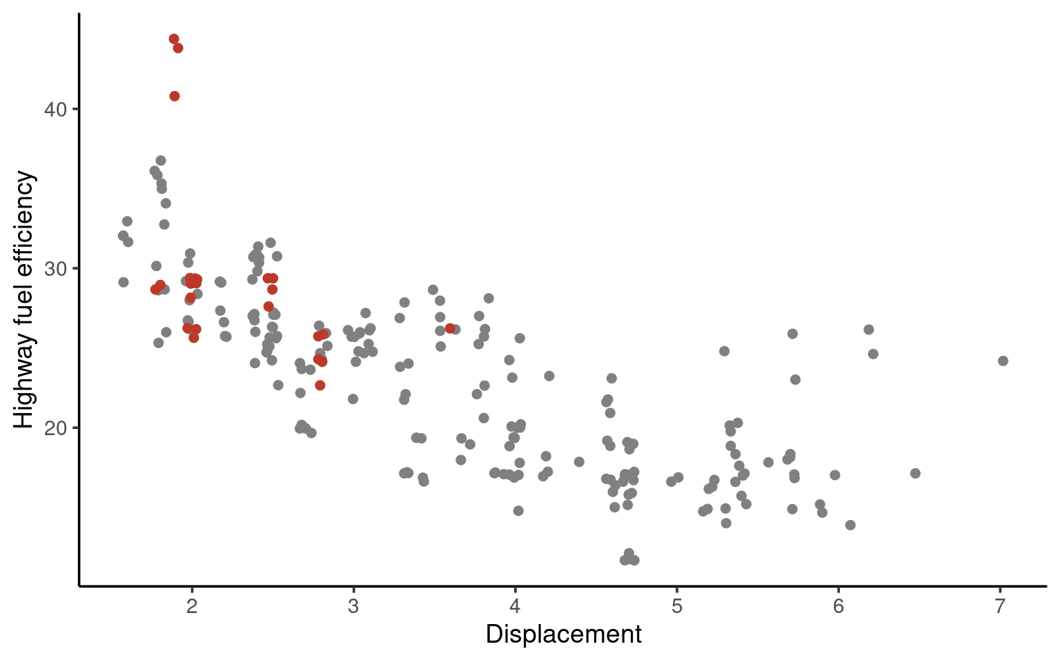
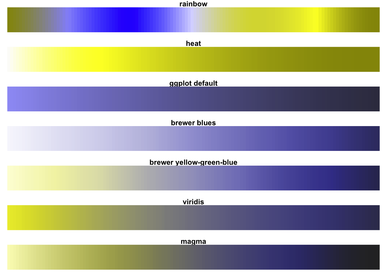
Humans cannot reason well about the RGB color space
Explore HCL colors with colorspace::choose_color()
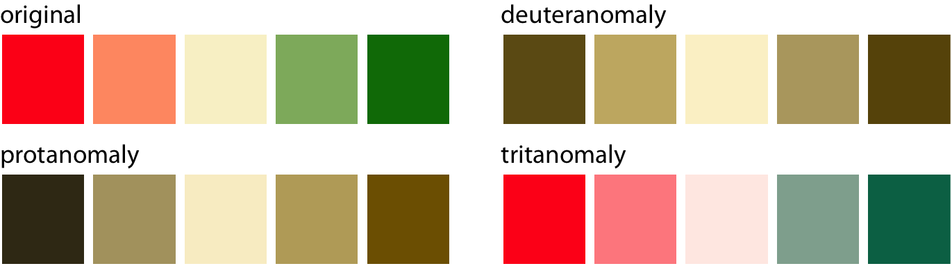
5%–8% of men are color blind!
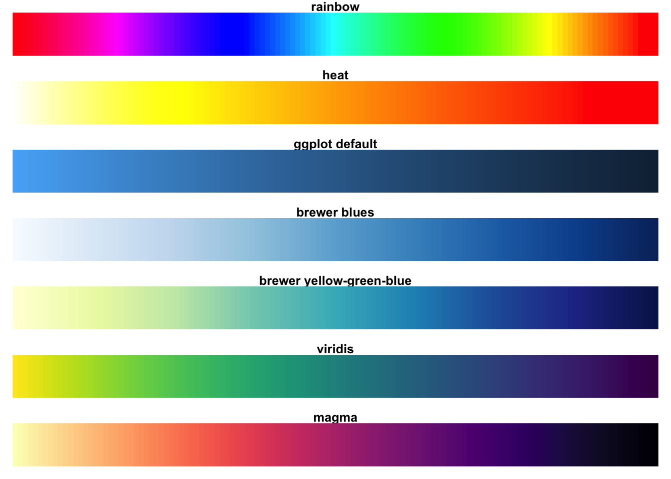
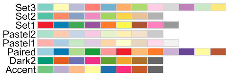
scale_color_brewer()
mpg |>
ggplot(aes(x = displ, y = hwy, color = drv)) +
geom_jitter() +
labs(x = "Displacement", y = "Highway fuel efficiency") +
scale_color_brewer(palette = "Accent") +
theme(legend.position = c(0.8, 0.8))
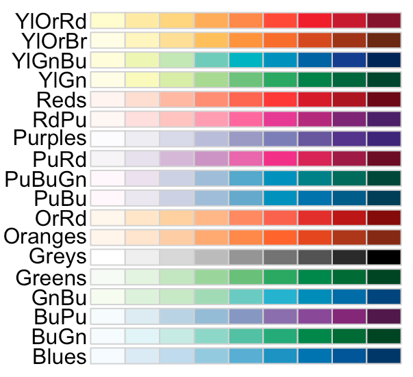
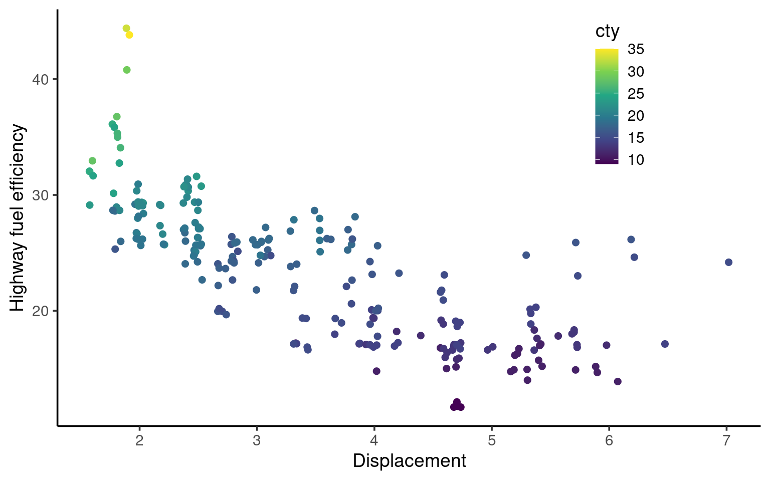
scale_color_distiller()
mpg |>
  ggplot(aes(x = displ, y = hwy, color = cty)) +
  geom_jitter() +
  labs(x = "Displacement", y = "Highway fuel efficiency") +
  scale_color_distiller(palette = "YlGnBu") +
  theme(legend.position = c(0.8, 0.8))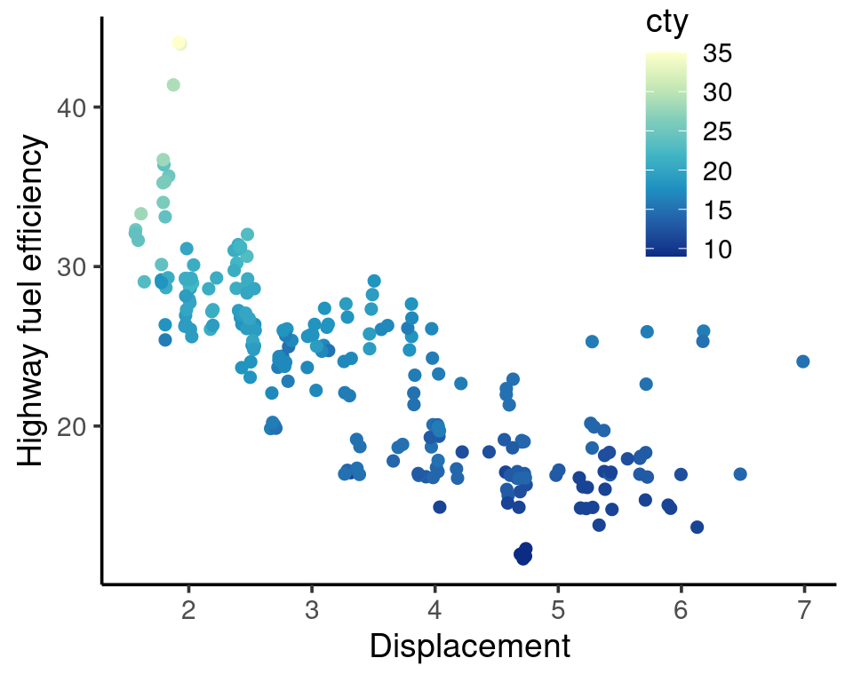
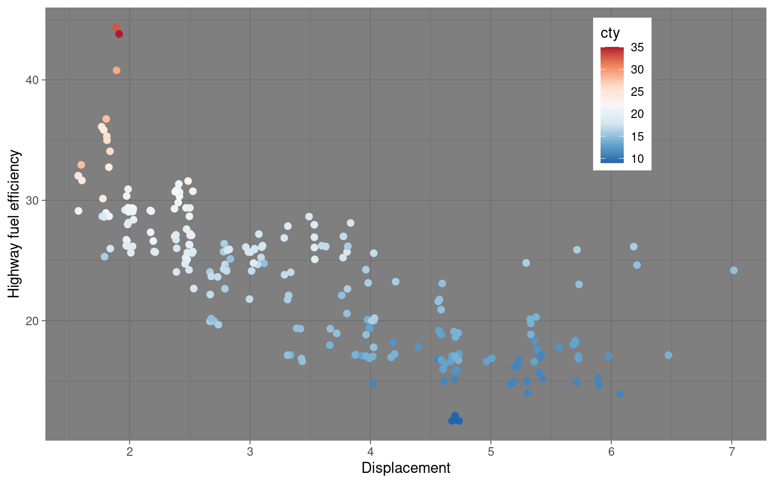
scale_color_distiller()
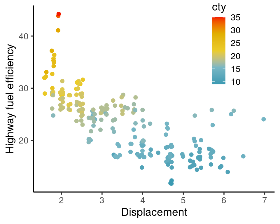
mpg |>
ggplot(aes(x = displ, y = hwy, color = cty)) +
geom_jitter() +
labs(x = "Displacement", y = "Highway fuel efficiency") +
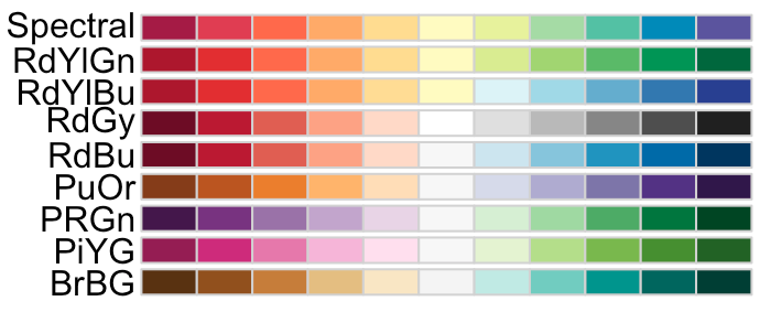
scale_color_distiller(palette = "Spectral") +
theme(legend.position = c(0.8, 0.8))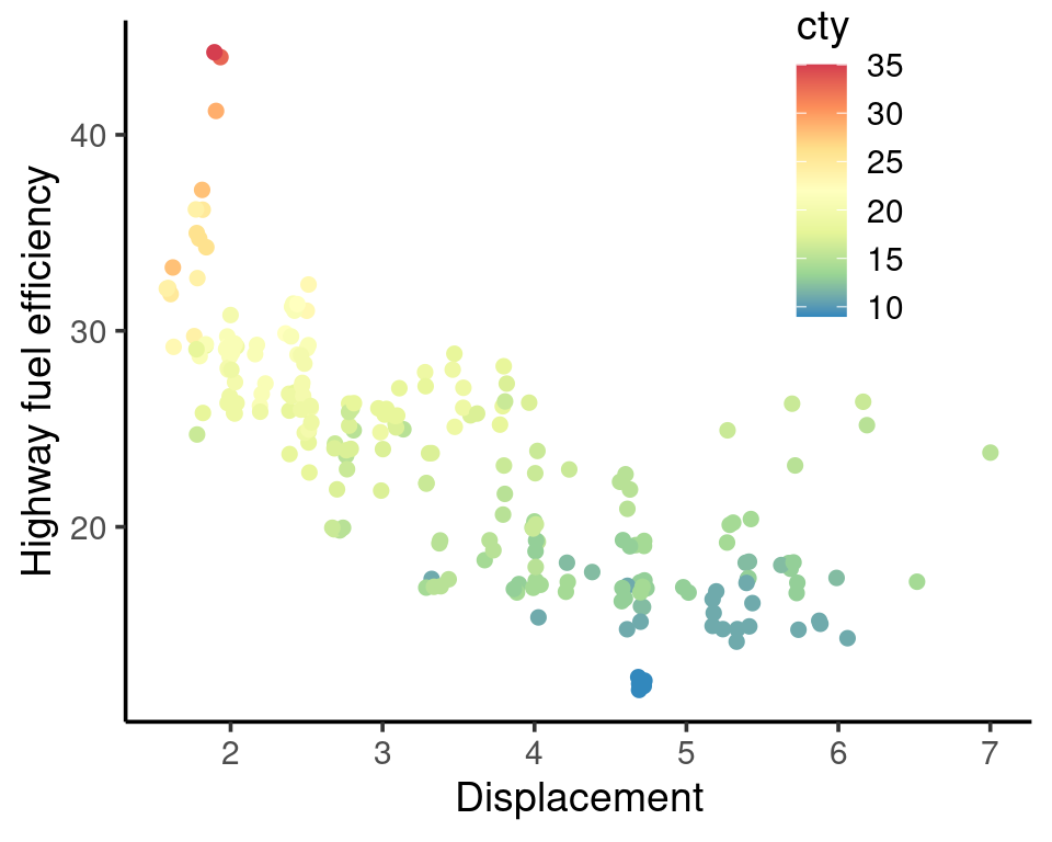


Switch to R script